Algorithm Engineering - Case Study: In one day to 3d cutting information system app
- Algorithm Engineering - Case Study: From Technical OR Problem to 3D Cutting System in One Day
- Executive Summary
- 1. The Technical OR Problem
- 2. Target System
- 3. System Architecture
- 4. Iteration 1: Batch-Capable Pipeline Instead of Demo Script
- 5. Iteration 2: Greedy Baseline and Rotation
- 6. Iteration 3: Saw Kerf as a Real Production Constraint
- 7. Iteration 4: Optimization Steering Above the Packing Core
- 8. Iteration 5: Layer-Packing 3D Optimization
- 9. Critical Bug: Batching Inside a Layer
- 10. Multi-Stage Validation
- 11. 3D Visualization as a Debugging and Communication Tool
- 12. Test Strategy
- 13. Example Results
- 14. What This Case Study Shows About R&D Engineering
- 15. Technical Lessons Learned
- 16. Result: An R&D Prototype With a Robust Pipeline
- 17. Conclusion
- Appendix A: Objective Function as an Engineering Model
- Appendix B: Validation Checklist
- Appendix C: Glossary
- Appendix C: Examples
summary: “This case study describes how an algorithm expert developed a 3D cutting system for orthogonal cutting-stock problems within a compact R&D sprint: from CSV batch processing, kerf modeling, strip-packing algorithms, and optimization control to 3D visualization, tests, and geometric validation.”
Algorithm Engineering - Case Study: From Technical OR Problem to 3D Cutting System in One Day
How a technical operations research problem became a working prototype for orthogonal 3D cutting
Hint: this is a Sces Study to Check AI Possibilities. The real Product is already in Production , see : https://softwareengel.de/verbesserung-bei-stahl-zuschnitt-durch-anpassung-und-integration-der-3d-verschnitt-optimierung/
Executive Summary
An algorithm expert receives a classic but very real industrial problem: given 3D parts must be cut from available raw blocks. The cuts are orthogonal, parts may be rotated, saw loss must be considered, and the result should be exportable as a production-oriented cutting plan.
Within a compact R&D sprint, this became a working 3D cutting system with:
- CSV batch processing for orders and raw materials
- Greedy baseline for fast results
- Layer/strip packing with a 0/1 knapsack component
- Saw kerf modeling
- multi-stage geometric validation against overlaps and container bounds
- 3D visualization as PNG and interactive Matplotlib view
- unit test suite for examples, algorithms, kerf, visualization, and bounds validation
- CLI workflow for repeatable production runs
The work shows how a hard operations research problem can be pragmatically translated into a robust engineering artifact: not by trying to build the mathematically perfect solver immediately, but through a controlled combination of heuristics, dynamic programming, validation, and test-driven iteration.
1. The Technical OR Problem
The underlying problem belongs to the family of multidimensional bin-cutting and bin-packing problems. In this case study, we consider a 3D variant:
- There is a set of orders
I. - Each order
iis a cuboid with dimensions(l_i, w_i, h_i). - There is a set of raw blocks
B. - Each raw block
bis a cuboid with dimensions(L_b, W_b, H_b). - An order may be placed in orthogonal rotations.
- Placements must not overlap.
- Every placement must lie completely inside a raw block.
- Material is lost between cuts because of the saw kerf.
- Unplaced orders must be penalized heavily.
1.1 Orthogonal 3D Cutting
In orthogonal cutting, all cuts are axis-aligned. A placed part is therefore described by the following values:
placement_i = (block_id, x_i, y_i, z_i, l_i', w_i', h_i')
Here, (x_i, y_i, z_i) is the lower-left-back corner inside the raw block, and (l_i', w_i', h_i') is a valid rotation of the original dimensions.
The simple bounds constraints are:
0 <= x_i
0 <= y_i
0 <= z_i

x_i + l_i' <= L_b
y_i + w_i' <= W_b
z_i + h_i' <= H_b
For every pair of placed parts i and j in the same raw block, a non-overlap condition must also hold. At least one of the following relations must be true:
i is left of j:       x_i + l_i' <= x_j
i is right of j:      x_j + l_j' <= x_i
i is in front of j:   y_i + w_i' <= y_j
i is behind j:        y_j + w_j' <= y_i
i is below j:         z_i + h_i' <= z_j
i is above j:         z_j + h_j' <= z_i
Even without additional production constraints, this is already a difficult combinatorial problem. In practice, more requirements are added: saw loss, cutting plans, robust reports, visual inspection, runtime limits, and understandable error messages.
2. Target System
The goal was not an academic paper solver, but an R&D prototype close to production use:
-
Data in: orders and raw blocks as CSV.
-
Run algorithm: greedy or layer-inspired packing.
-
Result out: cutting plan, report, visualization.
-
Check quality: unit tests, volume conservation, bounds, no overlap.
-
Ensure iteration: CLI, reproducible examples, clear project structure.
The key engineering principle was: first build a correct pipeline, then improve optimization.
3. System Architecture
The final architecture can be described in six layers.
┌──────────────────────────────────────────────┐
│ CLI / Batch Workflow                         │
│ orders.csv + raw_blocks.csv + options        │
└──────────────────────────────────────────────┘
                    │
┌──────────────────────────────────────────────┐
│ Input / Output Layer                         │
│ CSV loader, cut_plan.csv, report.txt, PNG    │
└──────────────────────────────────────────────┘
                    │
┌──────────────────────────────────────────────┐
│ Packing Core                                 │
│ Greedy baseline + rotations + free spaces    │
└──────────────────────────────────────────────┘
                    │
┌──────────────────────────────────────────────┐
│ Optimization Steering                        │
│ assignment strategies, scoring, caching      │
└──────────────────────────────────────────────┘
                    │
┌──────────────────────────────────────────────┐
│ Layer Packing                                │
│ layer heights, strip packing, knapsack DP    │
└──────────────────────────────────────────────┘
                    │
┌──────────────────────────────────────────────┐
│ Validation & Visualization                   │
│ bounds, overlap, volume conservation, 3D plots│
└──────────────────────────────────────────────┘
4. Iteration 1: Batch-Capable Pipeline Instead of Demo Script
The first step was converting an interactive demo optimizer into a batch-capable software component.
4.1 Input Format
The same CSV schema was deliberately used for orders and raw blocks:
id,length,width,height
ORD-001,20,15,10
ORD-002,25,20,12
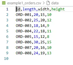
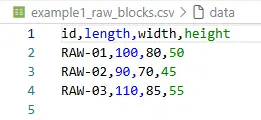
This reduces cognitive load and makes examples easy to generate.
4.2 Output Formats
The batch run creates three central artifacts:
<prefix>_cut_plan.csv
<prefix>_report.txt
<prefix>_<RAW-ID>_layout.png
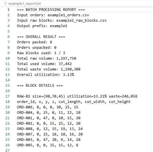
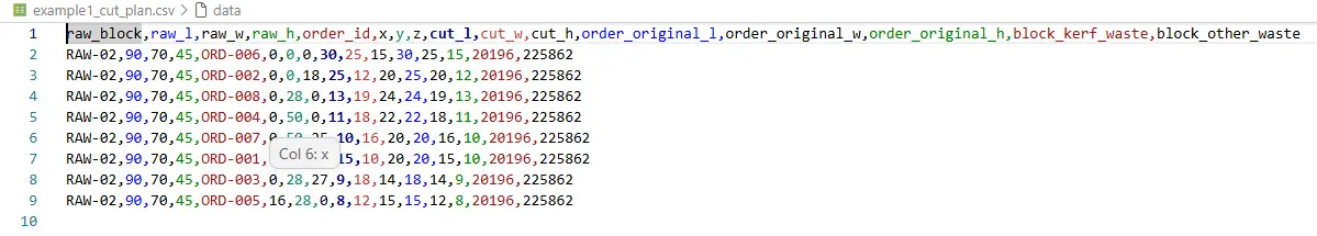
The cut_plan.csv is intended for downstream production or CNC-oriented processes. It contains:
-
raw block ID and raw block dimensions
-
order ID
-
placement coordinates
(x, y, z) -
cut dimensions
-
original dimensions for traceability
-
later added: kerf and remaining-material metrics
This turned the algorithm into a repeatable batch process.
5. Iteration 2: Greedy Baseline and Rotation
In operations research, a robust baseline is often more valuable than an immature meta-solver. The greedy variant works according to the following principle:
-
Sort orders by volume.
-
Try all orthogonal rotations for each order.
-
Find a suitable free space.
-
Place the part.
-
Split the remaining space guillotine-style into new free spaces.
-
Repeat until no further placement is possible.
5.1 Why Greedy First?
Greedy is not globally optimal, but it is:
-
fast
-
deterministic
-
easy to test
-
a good comparison baseline
-
helpful for regression tests
In the early examples, this baseline already delivered usable results, such as complete packings for small and medium datasets.
6. Iteration 3: Saw Kerf as a Real Production Constraint
A theoretical packing without saw loss is misleading in manufacturing. For that reason, the saw kerf was explicitly modeled.
6.1 Modeling Decision
For every placement, material loss is estimated through cut surfaces:
kerf_loss = (l × w + l × h + w × h) × saw_width
In addition, the free-space split reserves distance for the saw kerf, so neighboring parts are not unrealistically planned edge-to-edge without material loss.
6.2 Volume Balance
After introducing the kerf, the volume equation had to be adjusted:
total_volume = used_volume + kerf_waste + other_waste
This simple equation became a central test criterion. It prevents material from “disappearing” or being counted twice because of calculation errors.
7. Iteration 4: Optimization Steering Above the Packing Core
A single greedy run only answers the question: “What happens with this order?”
The actual production problem asks: “Which assignment of orders to raw blocks is better overall?”
For this, an optimization steering layer was placed above the packing core.
7.1 Strategies
The steering layer generates multiple candidate solutions, for example:
-
sorting by largest dimension
-
sorting by smallest dimension
-
sorting by surface area
-
sorting by aspect ratio
-
random, reproducible shuffles
-
round-robin assignment
-
size-based block affinity
7.2 Deduplication
Many strategies can produce the same effective assignment. Therefore, a hash-based cache system was introduced:
assignment_hash = hash(order_id -> block_id)
This detects duplicate solutions, skips them, and reduces runtime.
7.3 Scoring
The evaluation of a solution combines several objectives:
score =
    utilization_weight
  - blocks_used_penalty
  - unpacked_orders_penalty
  - waste_variance_penalty
  - kerf_penalty
An important bug fix was to avoid penalizing raw volume values in millions of cubic millimeters directly. Instead, the values had to be normalized. Only then did the scores become interpretable again, and the steering layer could reliably reject worse solutions.
8. Iteration 5: Layer-Packing 3D Optimization
For more demanding cases, a layer-packing method was implemented. The approach uses ideas from the container-loading problem and combines them with pragmatic Python optimizations.
8.1 Algorithmic Building Blocks
The implemented approach consists of:
-
Layer Packing
The raw block is split into layers along the z-axis. -
Box Rotation & Pairing
Parts are rotated for a layer height. Compatible parts can be paired to better use layer heights. -
Recursive Strip Packing
A 2D layer is recursively split into strips. -
0/1 Knapsack per Strip
Within a strip, a dynamic programmer decides which boxes best fill the strip. -
Integration Layer
A conversion module mediates between the existing optimizer data model and the layer-packing data structures.
8.2 Simplified Pseudocode Model
function pack_orders_layer(orders, raw_blocks):
    remaining = orders

    for block in raw_blocks:
        z = 0

        while z < block.height and remaining not empty:
            layer_height = choose_layer_height(remaining, block, z)
            candidates = select_candidate_boxes(remaining, limit=MAX_BOXES_PER_LAYER)

            prepared = rotate_and_pair(candidates, layer_height)
            placements = pack_layer_with_strips(prepared, block.length, block.width, z)

            valid = validate_bounds(placements, block)

            commit(valid)
            remove_committed_orders(remaining)

            z += layer_height

    return blocks, remaining_as_unpacked
8.3 Why Not a Fully Exact Solver?
A full branch-and-bound approach can quickly become too slow in Python. The decision therefore favored a hybrid approach:
-
adopt core ideas from layer packing
-
control runtime through limits
-
enforce correctness through validation
-
keep improvements measurable and testable
The result is not a mathematical proof of optimality, but an R&D-ready optimizer with clean error control.
9. Critical Bug: Batching Inside a Layer
A particularly instructive error appeared while scaling the layer-packing-inspired method.
9.1 The Error
To control runtime, boxes were packed in batches. However, the faulty variant executed multiple packing calls inside the same layer:
while remaining_to_pack:
    batch = remaining_to_pack[:MAX_BOXES_PER_ATTEMPT]
    placements, waste = pack_layer_simple(...)
    all_placements.extend(placements)
All batches started at the same layer coordinates. As a result, multiple parts could occupy the same space or extend beyond the block boundary.
9.2 The Fix
The fix was to allow only one packing call per layer and instead limit the candidate set per layer:
boxes_for_layer = all_boxes_to_pack[:MAX_BOXES_PER_LAYER]

placements, waste = pack_layer_simple(
    boxes=boxes_for_layer,
    layer_width=block.box.l,
    layer_depth=block.box.w,
    layer_z=current_z,
    layer_height=layer_height
)
This is a classic R&D lesson: performance optimization must not violate the geometric semantics of the problem.
10. Multi-Stage Validation
After the batching bug, validation was deliberately designed to be redundant.
10.1 Validation During Strip Packing
Every placement candidate is checked against the container bounds:
px >= 0
py >= 0
z  >= 0

px + length <= container_l
py + width  <= container_w
z  + height <= container_h
Invalid placements are not added to the candidate solution in the first place.
10.2 Validation in the Integration Layer
When converting back into the main data model, the system checks again whether the placement lies inside the raw block.
10.3 Post-Processing Validation
A standalone tool validates the exported cut_plan.csv. This is important because this exact artifact may later be used in production or visualization processes.
The three validation stages are:
1. During search: avoid invalid candidates
2. Before commit: catch invalid placements
3. After export: independently validate the cutting plan
This turns an experimental algorithm into a robust system artifact.
11. 3D Visualization as a Debugging and Communication Tool
Visualization was not merely “nice to have.” It served three functions:
-
Debugging: Overlaps and bounds errors are visually easy to detect.
-
Validation: Stakeholders can understand cutting plans.
-
Communication: R&D results become tangible.
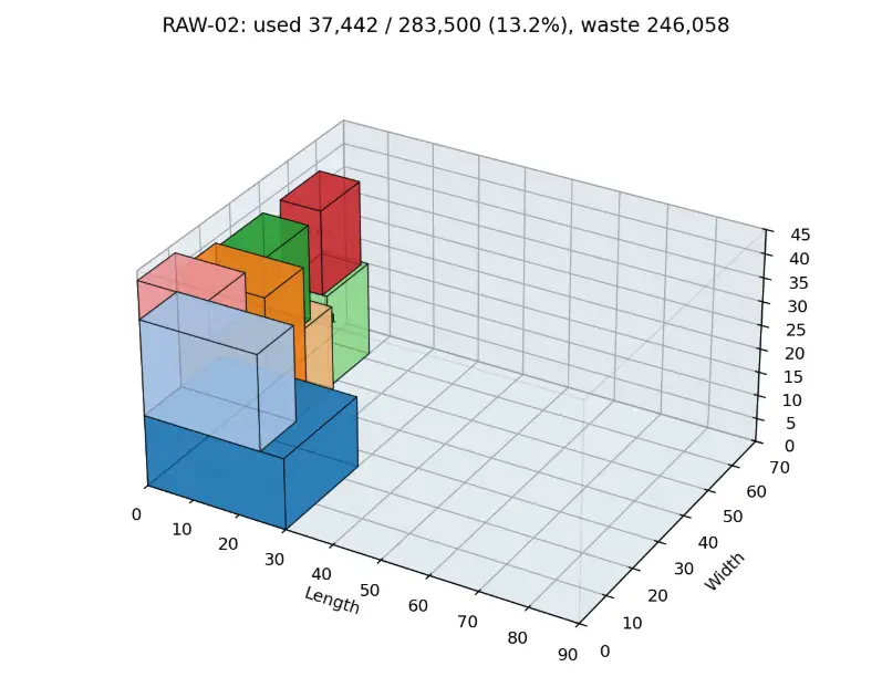
11.1 Visualization Elements
The 3D plots show:
-
transparent raw-block wireframes
-
colored order cuboids
-
order ID labels
-
utilization, leftover, and kerf metrics
-
summaries across all used blocks
11.2 Batch Output
For one run, the following files are created:
3d_plots/
├── example_RAW-01.png
├── example_RAW-02.png
└── example_summary.png
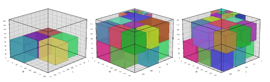
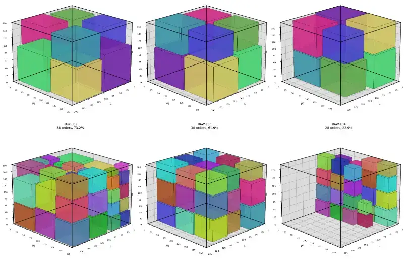
For larger examples, multiple block plots plus a summary plot were generated. This makes the cutting plan visually inspectable without manually analyzing the CSV.
12. Test Strategy
The test strategy was extended step by step.
12.1 Early Tests
The first suite validated:
-
CSV loading
-
number of loaded orders and raw blocks
-
number of packed and unpacked orders
-
volume calculations
-
utilization
-
no overlaps
-
bounds
-
volume conservation
12.2 Kerf Tests
After introducing the saw kerf, tests were added for:
-
positive kerf waste when
saw_width > 0 -
no kerf loss when
saw_width = 0 -
correct volume balance including kerf
-
capacity reduction caused by the saw kerf
12.3 Layer-Packing Tests
Separate tests were created for the layer-packing-inspired components:
-
knapsack solver
-
box preparation
-
box rotation
-
pairing
-
strip packing
-
integration
-
prevention of duplicate placements
12.4 Visualization Tests
Visualization was also made testable:
-
generation of box faces
-
color generation
-
PNG output
-
summary plot
-
large datasets
-
cases with unpacked orders
The result is a test chain that makes algorithmic and geometric errors visible early.
13. Example Results
The following results come from the development and validation runs of the system. They are not universal benchmarks, but they show that the pipeline works for cases of different sizes.
| Example | Orders | Raw Blocks | Result |
|---|---|---|---|
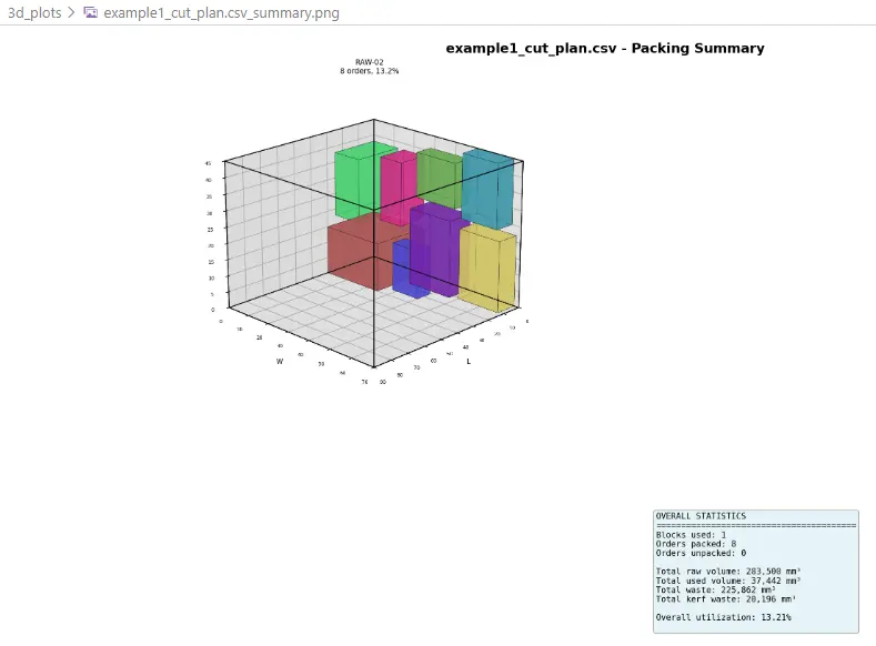
| Example 1 | 8 | 3 | 8/8 packed, 1 block used, approx. 3.13% total utilization |
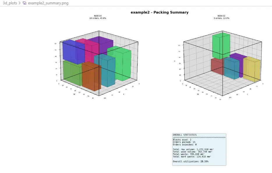
| Example 2 | 15 | 5 | 15/15 packed, 2 blocks used, approx. 9.24% total utilization |
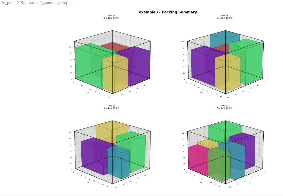
| Example 3 | 25 | 4 | depending on configuration, some orders remain unpacked; well suited as a stress case |
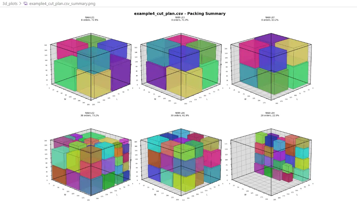
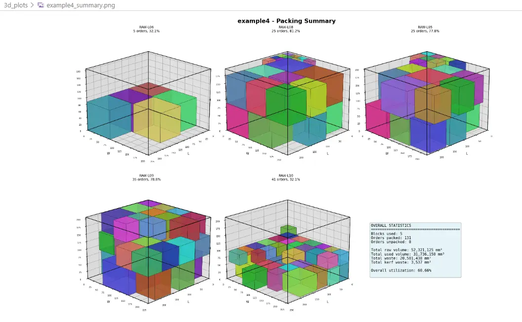
| Example 4 | 131 | 10 | after bounds fix, 131/131 packed, 5 blocks used, 35.54% utilization |
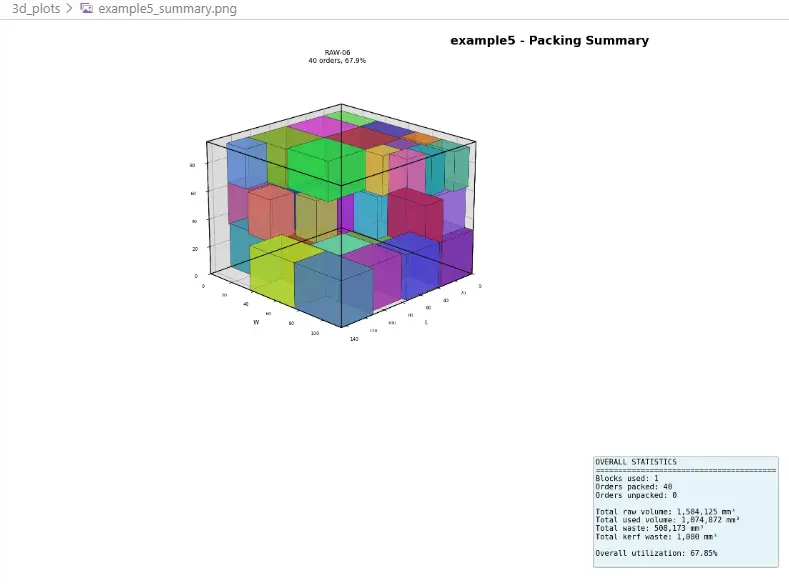
| Example 5 | 40 | 6 | after bounds fix, 40/40 packed, 1 block used, 8.19% utilization |
The low total utilization values in individual examples are not an error: if the available raw-block volume is significantly larger than the order volume, global utilization is naturally low. More meaningful is the combination of:
-
number of fully fulfilled orders
-
number of used raw blocks
-
utilization per used block
-
material loss caused by kerf
-
correctness of placements
14. What This Case Study Shows About R&D Engineering
14.1 A Hard Problem Becomes Manageable Through Layering
Instead of immediately building a monolithic solver, the problem was split into layers:
I/O → Greedy → Steering → Layer components → Validation → Visualization
Each layer delivered value on its own.
14.2 Correctness Is More Important Than Apparent Optimization
A fast algorithm that places parts outside the raw block is worthless. Only bounds validation made the system robust.
14.3 Visualization Accelerates Research
3D plots are not just presentation material. They are a debugging instrument for spatial algorithms.
14.4 Tests Are Part of the Algorithm
In geometric optimization, it is not enough to test function calls. Invariants must be tested:
no overlap
inside bounds
correct volume balance
no duplicate orders
unpacked orders explicitly reported
14.5 Heuristics Plus Validation Beats Naive Exactness
For an R&D prototype, a controlled heuristic solver is often more productive than an overly slow exact approach. What matters is that the heuristic does not hide its errors.
15. Technical Lessons Learned
Lesson 1: Normalize Before Scoring
A score that directly combines raw volumes in cubic millimeters with small penalty values can become numerically meaningless. Normalized metrics make the objective function interpretable.
Lesson 2: Respect Layer Semantics
Batching must not create multiple independent coordinate systems inside the same geometric layer. A layer needs exactly one consistent packing call or an explicit subspace model.
Lesson 3: Redundant Validation Is Not Overhead, but a Safety Net
Checking the same bounds rule in multiple places may seem redundant. In an optimization system with several conversion layers, however, it is the difference between debugging and trust.
Lesson 4: A Good Baseline Solver Remains Valuable
Even after introducing layer-packing-inspired components, greedy remains important:
-
as a fallback
-
as a comparison
-
as a fast plausibility check
-
as a regression test
Lesson 5: Production Readiness Starts With File Formats
CSV in, CSV/report/PNG out: this simple decision made the system immediately usable, testable, and explainable.
16. Result: An R&D Prototype With a Robust Pipeline
At the end of the sprint, the result was not a theoretical optimum, but a functional 3D cutting system:
python main.py example1_orders.csv example1_raw_blocks.csv example1 \
  --saw-width 3 \
  --visualize \
  --verbose
Or for optimized runs:
python main.py example3_orders.csv example3_raw_blocks.csv example3_optimized \
  --optimize \
  --max-time 30 \
  --max-iter 50 \
  --saw-width 3 \
  --visualize
The system can load order data, select raw blocks, calculate 3D placements, account for saw loss, export cutting plans, generate visualizations, and geometrically validate its results.
17. Conclusion
This case study shows how an algorithm expert can translate a complex technical OR problem into software within a very short time window.
The key was not a single brilliant algorithm, but the combination of:
-
clean problem formulation
-
fast greedy baseline
-
layer-packing-inspired optimization components
-
realistic manufacturing constraints such as kerf
-
consistent validation
-
visualization
-
automated tests
-
iterative debugging
The result is a pattern for modern R&D software development: scientifically inspired, pragmatically implemented, and secured against reality through tests.
Appendix A: Objective Function as an Engineering Model
A production-oriented objective function can be modeled as follows:
maximize score =
    α × utilization
  - β × used_blocks
  - γ × unpacked_orders
  - δ × normalized_waste_variance
  - ε × kerf_ratio
Typical priority:
-
No unpacked orders
-
No invalid placements
-
Fewer raw blocks
-
Better utilization
-
Less kerf
-
More even distribution of remaining material
Important: invalid placements should never merely be “penalized.” They must be excluded.
Appendix B: Validation Checklist
Before publishing a cutting plan, the system should check:
-
All placement coordinates are non-negative.
-
Every part lies completely inside the raw block.
-
No two parts overlap.
-
Every order ID is packed at most once.
-
Unplaced orders are explicitly reported.
-
used + kerf + waste = total. -
The CSV cutting plan can be validated independently.
-
The 3D visualization shows the same solution as the CSV export.
Appendix C: Glossary
3D Cutting Problem
Optimization problem in which three-dimensional parts are cut from three-dimensional raw material.
Bin Packing
Problem class in which objects are packed into as few containers as possible.
Bin Cutting
Related problem class focused on cutting, material loss, and cutting plans.
Kerf
Material loss caused by the width of the saw blade or cutting tool.
Guillotine Cut
A cut that passes completely through a remaining material piece.
Strip Packing
2D packing method in which an area is divided into strips.
0/1 Knapsack
Optimization problem in which a subset of objects is selected under a capacity constraint to maximize value.
Bounds Validation
Check whether placed geometries lie completely within their container bounds.
Utilization
Ratio of used material volume to available raw material volume.
Appendix C: Examples
Example 1 - 3D Cutting Summary
Example 2 - 3D Cutting Summary
Example 3 - 3D Cutting Summary
Example 4 - 3D Cutting Summary
Example 4b - 3D Cutting Summary
Example 5 - 3D Cutting Summary